
Fishnets, Honeycombs and Footballs – Better spatial models with hexagonal grids.
I love the unique mathematical properties of hexagonal tiling for spatial analysis and the inherent possibility to create beautiful bi-variate hex maps.
3rd March 2017 • Team Thoughts

GEOLYTIX asked me to share some of my thoughts about hex grids. What makes them special and why are they better suited for all aspects of our work than fishnets. There will be an in-depth look at the design of hex maps with Leaflet and Openlayers in a series of future blog posts and I am planning to do a workshop at FOSS4G 2017 in Boston. In this post I want to give a brief overview of regular grid sampling and the benefits of hexagonal grids over rectangular grids.
Hexagons are the closest shape to a circle that can form a regular grid.
Regular tiling of an Euclidean surface (eg. a map) can be achieved with triangles, squares (fishnets), or hexagons. The latter two can be further tessellated into triangles. But why is hexagonal tessellation best for maps?
The honeycomb conjecture itself was only proven in 1999 by American mathematician Thomas C. Hales. There is however plenty of accessible material on the nature of hex structures. My favourite is this TED.ed video.
It all boils down to the high perimeter / area ratio. Structural strength. That which is good for physical models should be good for an analytical model as well. But how does the need for less bee wax relate to making better maps? A map is a Cartographic (flat) representation of a distinct part of the spherical Earth. We must therefore flatten its surface in order for features to be drawn on a flat screen.

We ain’t going back to make you use cathode ray tubes for our web maps but fewer edges mean that less material needs to be bend when we put a hexagonal grid over a curving surface.
Think about the white bits on a golden age football.
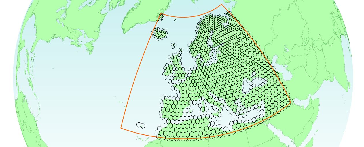
Every point on the surface of a hexagon is on average closer to the centre compared with points in a triangle or rectangle. This causes less distortion of the shape. Here is a more relevant representation which shows a hexagonal grid on an azimuthal projection which uses the location of GEOLYTIX offices in London as centre.
For the scientifically minded there is a peer reviewed article from Birch et al on ‘Rectangular and hexagonal grids used for observation, experiment and simulation in ecology’.
Turning heterogeneous areas into regular grid surfaces
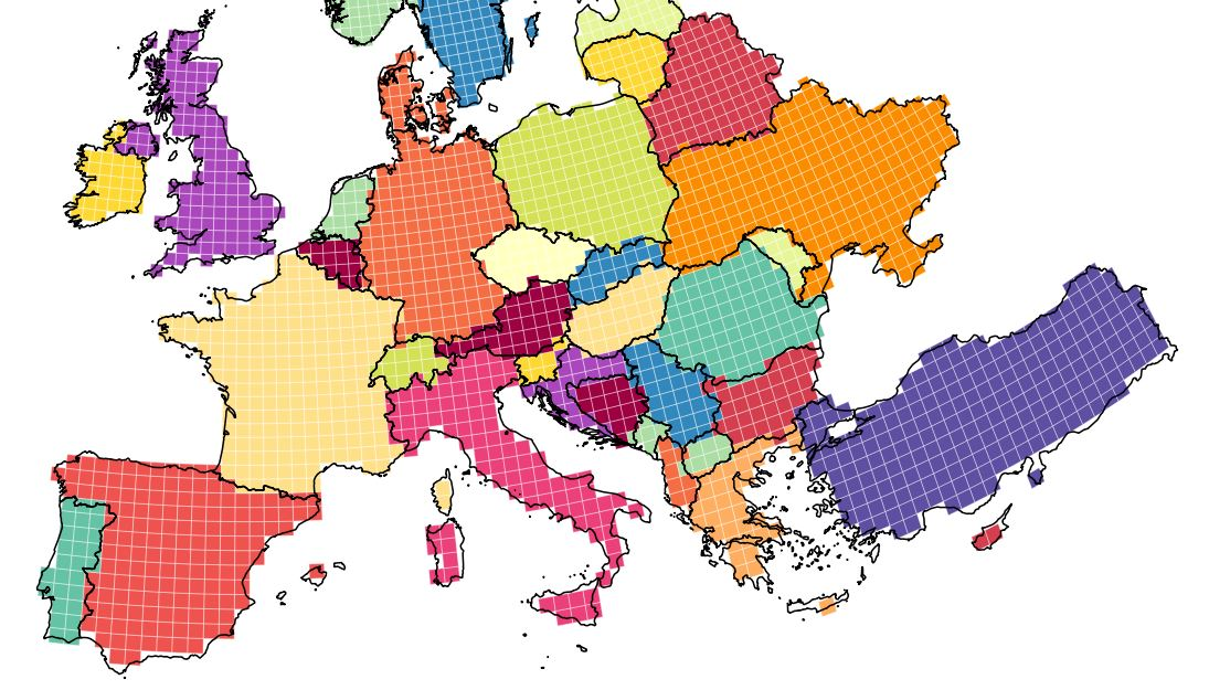
The next two grid maps show European countries split into equally sized hexagonal and rectangular grids.
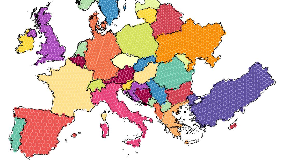
Apart from Luxembourg being completely ignored in the rectangular grid due a shape mismatch at the selected resolution it can be seen that the hexagonal grid matches the international boundaries better than the rectangular presentation.
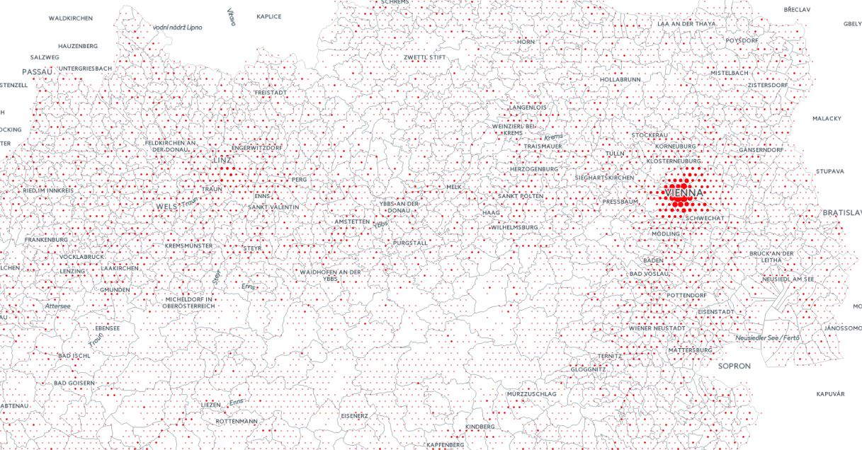
The next screenshot shows the distribution of registered unemployed in communities near Vienna. Very little variation can be seen in the rural communities outside the capital.
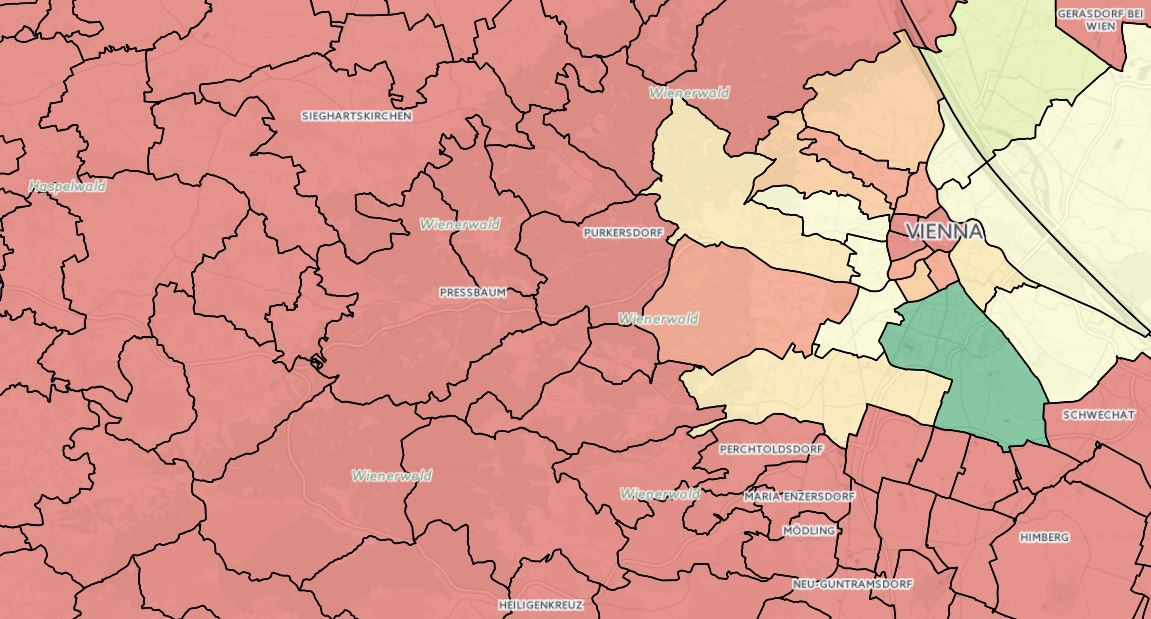
We get a much better insight into the actual distribution of unemployed labourers if we apply the figures from the communities to a hexagonal grid (1km cell height) which has been created from the Global Human Settlement (GHS) population grid. We see that large stretches of land are forests and do not represent the populated areas in which we are interested for a social model.
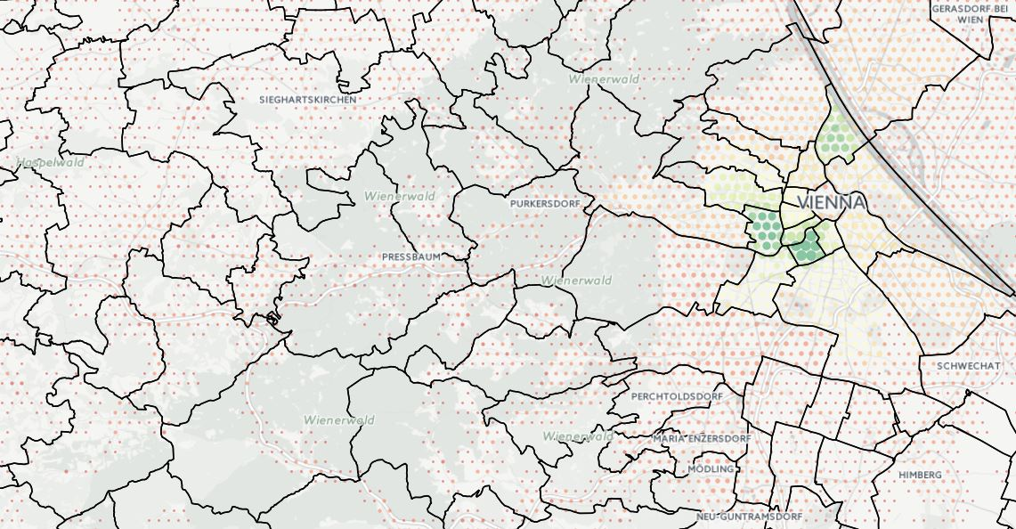
Unlike fixed reporting geometries, grid cells can be sized according to the required model scale. If we zoom out of the region shown in the images above we can no longer distinguish small urban communities. A hexagonal grid with 4km cell height however clearly shows the population distribution across the extended region.
Gridded networks
An important advantage of the hexagonal grid is the unambiguous definition of nearest neighbourhood: Each hexagon has six adjacent hexagons in symmetrically equivalent positions (Birch et al. 2000). In contrast, the rectangular
grid has two different kinds of nearest neighbour: orthogonal neighbours sharing an edge and diagonal neighbours sharing only a corner.
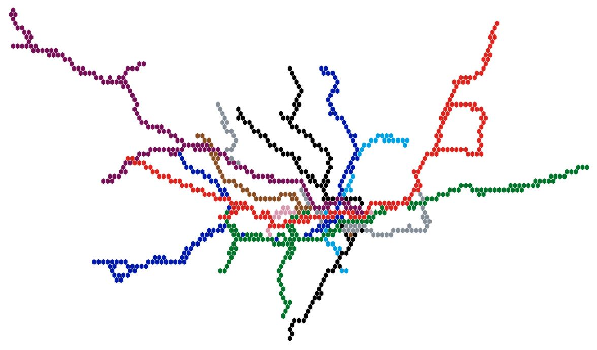
Networks can be better represented with a hexagonal grid. The next two images show the London Tube network as a rectangular grid, sometimes called a Manhatten grid, as well as a hexagonal grid. The colours represent the different tube lines.
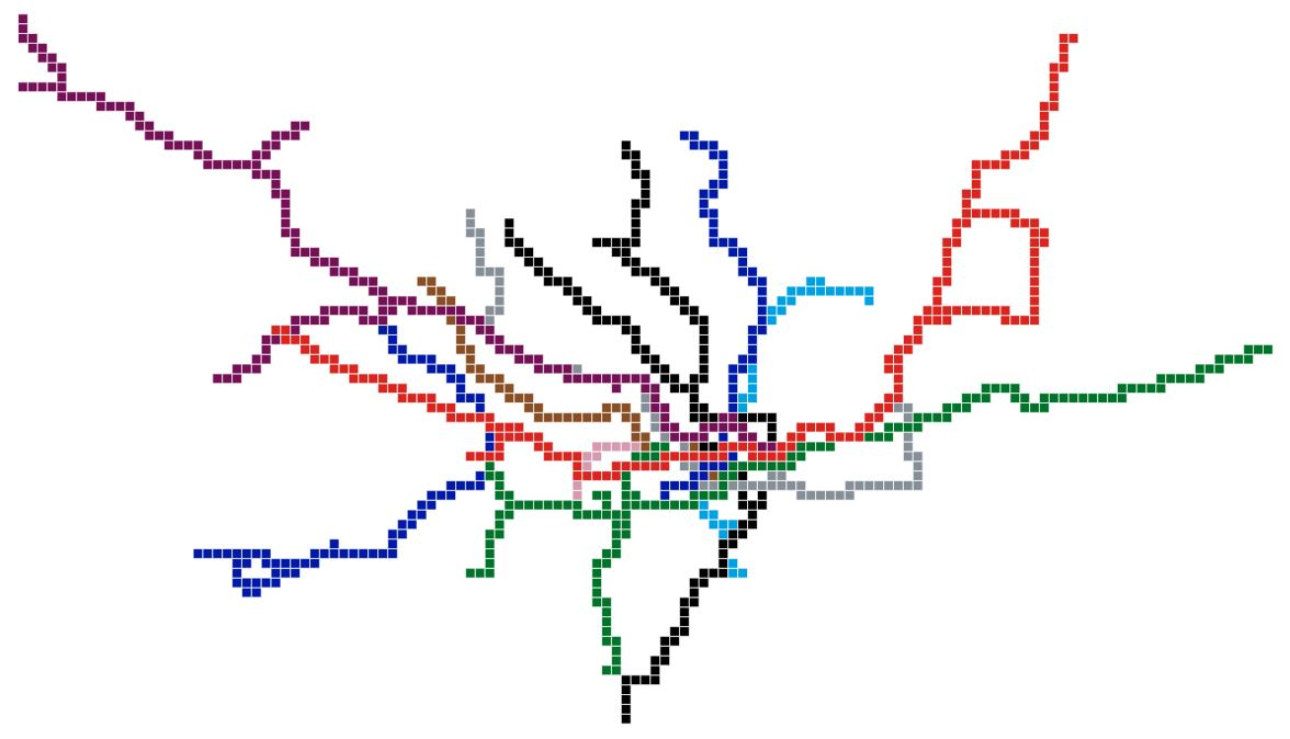
Being able to connect to diagonal neighbours improves the representation of the network in a hexagonal grid.
There are numerous blog posts which have pointed out the benefits of different types of grids. This post would not have been possible without the work and dedication of others. I want to point to this excellent gis.stackexchange post as well as this blog post by Matt Strimas-Mackey. Matt does some great work with R and highlights the square grid’s benefits of orthogonal simplicity and computational ease. With this in mind:

Related Posts
-

What’s the Catchment?
Catchments are more than just shapes on a map. Discover 7 ways to map your customers, analyse competitors, and optimise your location planning.
Published 26th May 2026 • Tags team-thoughts
-

Leeds and the 15-Minute City: A Retail Perspective
Leeds, the biggest city in Europe without a mass transit system. That is set to change. Freddie Wallace explores the benefits and challenges while evaluating the idea of a 15-minute city.
Published 10th March 2025 • Tags team-thoughts
-

The Importance of Site Visits for Location Planners
While data driven insights are essential, site visits are indispensable for Location Planning. Alison interviewed our Location Planners to find out why we do them and 10 top tips that might help you next time.
Published 1st June 2023 • Tags market-visits, team-thoughts